5. Reproducing Previous Results

This example recreates the results of Bryson et al. (2015) giving the same depths of formation of two pallasite meteorites.

As we’re setting this up step-by-step instead of using the pytesimal.quick_workflow module, we need to import a selection of modules:

import pytesimal.setup_functions
import pytesimal.load_plot_save
import pytesimal.numerical_methods
import pytesimal.analysis
import pytesimal.core_function
import pytesimal.mantle_properties

Instead of creating and loading a parameter file, we’re going to define variables here. The values are from and recreate the results of Bryson et al. (2015), with explanatory comments:

# These values are quoted in Bryson et al. (2015) or
# the references therein:

# material properties:
mantle_diffusivity = 5e-7
mantle_conductivity_value = 3.0
mantle_density_value = 3000.0

kappa_reg = 5e-8  # m^2/s

core_cp = 850.0  # J/(kg K)
core_density = 7800.0  # kg/m^3

# geometry:
r_planet = 200_000.0  # planetesimal radius in m
reg_m = 8_000.0  # megaregolith thickness in m

# temperatures:
temp_core_melting = 1200.0  # K
temp_init = 1600.0  # K
temp_surface = 250.0  # K
core_temp_init = 1600.0  # K
core_latent_heat = 270_000.0  # J/kg

# discretisation:
timestep = 2E11  # s
dr = 1000.0  # m
max_time = 400  # Myr

# This value isn't explicitly listed in Bryson et al., or references
# as Bryson et al. (2015) uses diffusivity instead
mantle_heatcap_value = mantle_conductivity_value / (mantle_density_value * mantle_diffusivity)

# Bryson et al. (2015) list regolith in km as opposed to
# as a fraction of body radius
reg_fraction = reg_m / r_planet  # fraction of r_planet

# We don't want to incorporate the 8 km regolith when calculating core size:
# Bryson et al. (2015) don't seem to include the regolith when calculating
# the core size, ie the core is 50% of the non-regolith body radius.
# We don't want to incorporate the 8 km regolith when calculating core size:
core_m = (r_planet - reg_m) * 0.5  # 100_000.0 # core size in m
core_size_factor = core_m / r_planet  # fraction of r_planet

The setup_functions.set_up() function creates empty arrays to be filled with resulting temperatures:

(r_core,
 radii,
 core_radii,
 reg_thickness,
 where_regolith,
 times,
 mantle_temperature_array,
 core_temperature_array) = pytesimal.setup_functions.set_up(timestep,
                                                            r_planet,
                                                            core_size_factor,
                                                            reg_fraction,
                                                            max_time,
                                                            dr)

# We define an empty list of latent heat that will
# be filled as the core freezes
latent = []

Next, we instantiate the core object. This will keep track of the temperature of the core as the model runs, cooling as heat is extracted across the core-mantle boundary. This simple eutectic core model doesn’t track inner core growth, but this is still a required argument to allow for future incorporation of more complex core objects:

core_values = pytesimal.core_function.IsothermalEutecticCore(
    initial_temperature=core_temp_init,
    melting_temperature=temp_core_melting,
    outer_r=r_core,
    inner_r=0,
    rho=core_density,
    cp=core_cp,
    core_latent_heat=core_latent_heat)

Then we define the mantle properties. The default is to have constant values, so we don’t require any arguments for this example:

(mantle_conductivity,
 mantle_heatcap,
 mantle_density) = pytesimal.mantle_properties.set_up_mantle_properties()

You can check (or change) the value of these properties after they’ve been set up using one of the MantleProperties methods. We want to set these values equal to the values used by Bryson et al. (2015):

mantle_conductivity.setk(mantle_conductivity_value)
mantle_heatcap.setcp(mantle_heatcap_value)
mantle_density.setrho(mantle_density_value)

You can check that the correct values have been assigned:

print(mantle_conductivity.getk())
print(mantle_heatcap.getcp())
print(mantle_density.getrho())

Out:

3.0
2000.0
3000.0

If temperature dependent properties are used, temperature can be passed in as an argument to return the value at that temperature.

We need to set up the boundary conditions for the mantle. For this example, we’re using fixed temperature boundary conditions at both the surface and the core-mantle boundary.

top_mantle_bc = pytesimal.numerical_methods.surface_dirichlet_bc
bottom_mantle_bc = pytesimal.numerical_methods.cmb_dirichlet_bc

(mantle_temperature_array,
 core_temperature_array,
 latent,
 ) = pytesimal.numerical_methods.discretisation(
    core_values,
    latent,
    temp_init,
    core_temp_init,
    top_mantle_bc,
    bottom_mantle_bc,
    temp_surface,
    mantle_temperature_array,
    dr,
    core_temperature_array,
    timestep,
    r_core,
    radii,
    times,
    where_regolith,
    kappa_reg,
    mantle_conductivity,
    mantle_heatcap,
    mantle_density)

This function fills the empty arrays produced by setup_functions.set_up() with calculated temperatures for the mantle and core.

Now we can use the pytesimal.analysis module to find out more about the model run. We can check when the core was freezing, so we can compare this to the cooling history of meteorites and see whether they can be expected to record magnetic remnants of a core dynamo:

(core_frozen,
 times_frozen,
 time_core_frozen,
 fully_frozen) = pytesimal.analysis.core_freezing(core_temperature_array,
                                                  max_time,
                                                  times,
                                                  latent,
                                                  temp_core_melting,
                                                  timestep)

Then, we can calculate arrays of cooling rates from the temperature arrays:

mantle_cooling_rates = pytesimal.analysis.cooling_rate(
    mantle_temperature_array,
    timestep)
core_cooling_rates = pytesimal.analysis.cooling_rate(core_temperature_array,
                                                     timestep)

Meteorite data (the diameter of ‘cloudy-zone particles’) can be used to estimate the rate at which the meteorites cooled through a specific temperature (C. W. Yang et al., 1997). The analysis.cooling_rate_cloudyzone_diameter function calculates the cooling rate in K/Myr, while the analysis.cooling_rate_to_seconds function converts this to K/s which allows comparison to our result arrays.

d_im = 147  # cz diameter in nm
d_esq = 158  # cz diameter in nm

imilac_cooling_rate = pytesimal.analysis.cooling_rate_to_seconds(
    pytesimal.analysis.cooling_rate_cloudyzone_diameter(d_im))
esquel_cooling_rate = pytesimal.analysis.cooling_rate_to_seconds(
    pytesimal.analysis.cooling_rate_cloudyzone_diameter(d_esq))

We can use this cooling rate information to find out how deep within their parent bodies these meteorites originally formed, and when they passed through the temperature of tetrataenite formation (when magnetism can be recorded). The analysis.meteorite_depth_and_timing() function returns the source depth of the meteorite material in the parent body based on the metal cooling rates at 800 K (as a depth from surface in km and as a radial value from the center of the planet in m), the time that the meteorite cools through the tetrataenite formation temperature in comparison to the core crystallisation period, and a string defining this relation between paleomagnetism recording and dynamo activity:

(im_depth,
 im_string_result,
 im_time_core_frozen,
 im_Time_of_Crossing,
 im_Critical_Radius) = pytesimal.analysis.meteorite_depth_and_timing(
    imilac_cooling_rate,
    mantle_temperature_array,
    mantle_cooling_rates,
    radii,
    r_planet,
    core_size_factor,
    time_core_frozen,
    fully_frozen,
    dr=1000,
    dt=timestep
)

(esq_depth,
 esq_string_result,
 esq_time_core_frozen,
 esq_Time_of_Crossing,
 esq_Critical_Radius) = pytesimal.analysis.meteorite_depth_and_timing(
    esquel_cooling_rate,
    mantle_temperature_array,
    mantle_cooling_rates,
    radii,
    r_planet,
    core_size_factor,
    time_core_frozen,
    fully_frozen,
    dr=1000,
    dt=timestep
)

print(f"Imilac depth: {im_depth}; Imilac timing: {im_string_result}")
print(f"Esquel depth: {esq_depth}; Esquel timing: {esq_string_result}")

Out:

Imilac depth: 38.0; Imilac timing: Core has not started solidifying yet
Esquel depth: 45.0; Esquel timing: Core has started solidifying

If you need to save the meteorite results, they can be saved to a dictionary which can then be passed to the load_plot_save.save_params_and_results. This allows for any number of meteorites to be analysed and only the relevant data stored:

meteorite_results_dict = {'Esq results':
                              {'depth': esq_depth,
                               'text result': esq_string_result},
                          'Im results':
                              {'depth': im_depth,
                               'text result': im_string_result,
                               'critical radius': im_Critical_Radius}}

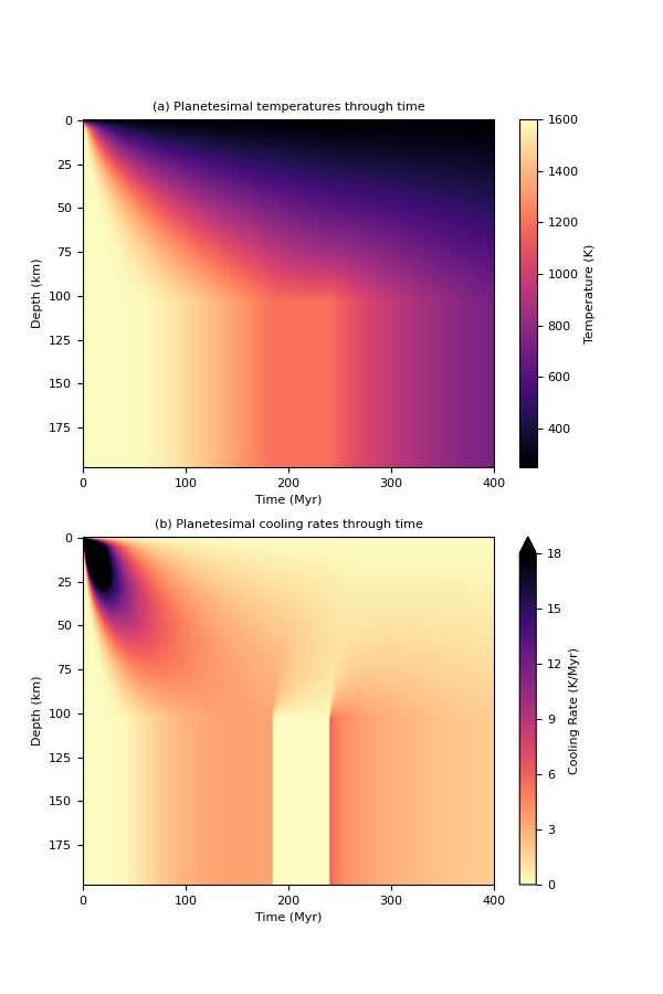
To get an overview of the cooling history of the body, it’s very useful to plot the temperatures and cooling rates as a heatmap through time. In order to plot the results, we need to define a figure height and width, then call load_plot_save.plot_temperature_history(), load_plot_save.plot_coolingrate_history() or load_plot_save.two_in_one(). These functions convert the cooling rate from K/timestep to K/Myr to make the results more human-readable.

fig_w = 6
fig_h = 9

pytesimal.load_plot_save.two_in_one(
    fig_w,
    fig_h,
    mantle_temperature_array,
    core_temperature_array,
    mantle_cooling_rates,
    core_cooling_rates,
    timestep=timestep)