Note
Click here to download the full example code
0. Introduction
Pytesimal is a finite difference code to perform numerical models of a conductively cooling planetesimal, both with constant and temperature-dependent properties.
In this example, we walk through the theoretical background of the model and explain step-by-step how the code works.
Model set-up
Pytesimal allows the modelling of a conductively cooling body, with the following different regions:
An isothermal convecting core: this can be replaced with a more complex core model or can be switched off to make a core-less body.
A discretised, conductive mantle: this is the region of focus in Pytesimal. The material properties for this region can be temperature-dependent or constant.
A discretised megaregolith: this region is also conductively cooling; material properties can only be constant in this region (constant diffusivity). This region can be switched off.
These different configurations, along with different material properties, can be set up to replicate a wide variety of different planetesimal geometries.
In order to set up our model, we first import the required packages:
import pytesimal.setup_functions
import pytesimal.load_plot_save
import pytesimal.numerical_methods
import pytesimal.analysis
import pytesimal.core_function
import pytesimal.mantle_properties
One way of setting up a model run is to use a parameter file. The parameter file is essentially a dictionary holding values for different variables, including the planetesimal radius, core size and regolith thickness, material properties for the body, and values to define the numerical discretisation.
We can generate a default parameter file by calling the make_default_param_file function. This function can be called with a filepath argument, specifying where the file should be saved and what it should be called:
filepath = 'parameters.txt'
pytesimal.load_plot_save.make_default_param_file(filepath)
This provides a template file for you to edit to suit your specific model set up (see documentation on parameter files for more information on the content and layout of the parameter file). This file can be edited and then loaded in - in practise, you wouldn’t do this all in one script like we have here - you would create and edit a parameter file (or copy and edit a pre-existing one), and then in a separate script, would load the parameter file and run the model.
As we’re just going to use the default values from the parameter file, we’ll just load it straight back in without editing it:
(run_ID, folder, timestep, r_planet, core_size_factor,
 reg_fraction, max_time, temp_core_melting, mantle_heatcap_value,
 mantle_density_value, mantle_cond_value, core_heatcap, core_density,
 temp_init, temp_surface, core_temp_init, core_latent_heat,
 kappa_reg, dr, cond_constant, density_constant,
 heat_cap_constant) = pytesimal.load_plot_save.load_params_from_file(filepath)
This big collection of parameters will be fed in to our model!
To make this example run a bit faster, we’re going to change the timestep from \(1 \times 10^{11}\) to \(2 \times 10^{11}\)
timestep = 2e11

#
# In order to discretise the different regions and record temperatures
# at radii points at each timestep, we need to set up some arrays
# that match the geometry we've passed in using the parameter file.
# These arrays will be placeholders until the numerical method fills
# them with values:

(r_core,
 radii,
 core_radii,
 reg_thickness,
 where_regolith,
 times,
 mantle_temperature_array,
 core_temperature_array) = pytesimal.setup_functions.set_up(timestep,
                                                            r_planet,
                                                            core_size_factor,
                                                            reg_fraction,
                                                            max_time,
                                                            dr)
The planetesimal core
Before we set up the numerical scheme for the discretised regions of the planetesimal, we need to instantiate the core object. This will keep track of the temperature of the core as the model runs, cooling as heat is extracted across the core-mantle boundary. The heat extracted in one timestep (\(P_{\mathrm{CMB}}\)) is:
where \(A_\mathrm{c}\) is the core surface area, \(r_\mathrm{c}\) is the core radius, and \(k_\mathrm{m}\) is the thermal conductivity at the base of the mantle or discretised region. The corresponding change in core boundary temperature \(\Delta T\) is:
where \(\rho_{\mathrm{c}}\) and \(C_{\mathrm{c}}\) are the density and heat capacity of the core, and \(V_{\mathrm{c}}\) is the volume of the core.
Once the core reaches its freezing temperature, the temperature is pinned. Latent heat is extracted until the total latent heat associated with core crystallisation has been removed. We need to set up an empty list to keep track of this latent heat:
latent = []
This simple eutectic core model doesn’t track inner core growth, but this is still a required argument to allow for future incorporation of more complex core objects:
core_values = pytesimal.core_function.IsothermalEutecticCore(initial_temperature=core_temp_init,
                                                             melting_temperature=temp_core_melting,
                                                             outer_r=r_core, inner_r=0, rho=core_density,
                                                             cp=core_heatcap,
                                                             core_latent_heat=core_latent_heat)
Conductive cooling
The conductively cooling regions in the planetesimal can be described in 1D by the heat equation in spherical geometry:
where \(T\) is temperature, \(t\) is time, \(\rho\) is density, \(C\) is heat capacity, \(k\) is thermal conductivity, and \(r\) is radius.
We need to define the thermal properties for this region (\(\rho\), \(C\), and \(k\)). In our parameter file, we’ve already defined these as constant in temperature and have listed values. We just need to pass those arguments to the set_up_mantle_properties function:
(mantle_conductivity, mantle_heatcap, mantle_density) = pytesimal.mantle_properties.set_up_mantle_properties(
    cond_constant,
    density_constant,
    heat_cap_constant,
    mantle_density_value,
    mantle_heatcap_value,
    mantle_cond_value)
The conduction equation is solved numerically using an explicit finite difference scheme, Forward-Time Central-Space (FTCS). FTCS gives first-order convergence in time and second-order in space, and is conditionally stable when applied to the heat equation. We can quickly calculate the diffusivity in the mantle and then check we meet Von Neumann stability criteria for the mantle and the megaregolith:
mantle_diffusivity = pytesimal.numerical_methods.calculate_diffusivity(mantle_cond_value, mantle_heatcap_value,
                                                                       mantle_density_value)

mantle_stability = pytesimal.numerical_methods.check_stability(mantle_diffusivity, timestep, dr)

reg_stability = pytesimal.numerical_methods.check_stability(kappa_reg, timestep, dr)
Out:
Von Neumann stability criteria met
Von Neumann stability criteria met
We set up the boundary conditions for the mantle. For this example, we’re using fixed temperature boundary conditions at both the surface and the core-mantle boundary: at the planetesimal’s surface, the temperature is held at a fixed temperature specified in the parameter file (250 K), while at the core-mantle boundary, the temperature is updated by the core.
top_mantle_bc = pytesimal.numerical_methods.surface_dirichlet_bc
bottom_mantle_bc = pytesimal.numerical_methods.cmb_dirichlet_bc
Now we pass our boundary conditions, core object, initial temperature, material properties, geometry, and arrays to the discretisation function, which returns arrays of temperatures in the mantle and the core, and a list of latent heat values during core crystallisation:
(mantle_temperature_array,
 core_temperature_array,
 latent,
 ) = pytesimal.numerical_methods.discretisation(
    core_values,
    latent,
    temp_init,
    core_temp_init,
    top_mantle_bc,
    bottom_mantle_bc,
    temp_surface,
    mantle_temperature_array,
    dr,
    core_temperature_array,
    timestep,
    r_core,
    radii,
    times,
    where_regolith,
    kappa_reg,
    mantle_conductivity,
    mantle_heatcap,
    mantle_density)
Analysing results
We can calculate the cooling rates in the planetesimal with the analysis module:
mantle_cooling_rates = pytesimal.analysis.cooling_rate(mantle_temperature_array, timestep)
core_cooling_rates = pytesimal.analysis.cooling_rate(core_temperature_array, timestep)
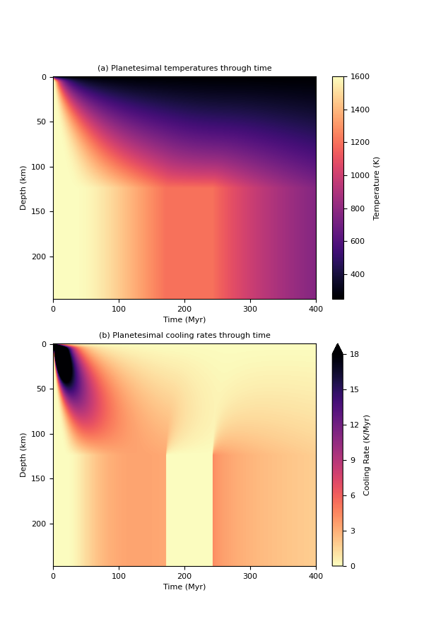
We can then plot the results using the load_plot_save module. The two_in_one function can be called to quickly plot both the temperature and cooling rates:
fig_w = 6
fig_h = 9

pytesimal.load_plot_save.two_in_one(
    fig_w,
    fig_h,
    mantle_temperature_array,
    core_temperature_array,
    mantle_cooling_rates,
    core_cooling_rates,
    timestep=timestep)
Further information
Other examples are available in the gallery, and further information on the theoretical background can be found in Murphy Quinlan et al. (2021).
Total running time of the script: ( 0 minutes 43.549 seconds)