4. Planetesimal Without a Core

This example shows step by step how to set up and run a model of a cooling planetesimal without a core. This example uses constant material properties in the mantle, see Murphy Quinlan et al. (2021) and references therein.

While the material properties used in this example are suitable for modelling the olivine mantle of a differentiated body, the model set-up may be useful for modelling undifferentiated meteorite parent bodies with appropriate thermal properties.

This model set-up also allows for comparison to an analytical solution for conductive cooling in a sphere (see Murphy Quinlan et al. (2021)).

As we’re setting this up step-by-step instead of using the pytesimal.quick_workflow module, we need to import a selection of modules:

import pytesimal.setup_functions
import pytesimal.load_plot_save
import pytesimal.numerical_methods
import pytesimal.analysis
import pytesimal.core_function
import pytesimal.mantle_properties

Instead of creating and loading a parameter file, we’re going to define variables here. The values match those of the constant thermal properties case in Murphy Quinlan et al. (2021), except for the core_size_factor value:

timestep = 1E11  # s
r_planet = 250_000.0  # m
reg_fraction = 0.032  # fraction of r_planet
max_time = 400  # Myr
temp_core_melting = 1200.0  # K
core_cp = 850.0  # J/(kg K)
core_density = 7800.0  # kg/m^3
temp_init = 1600.0  # K
temp_surface = 250.0  # K
core_temp_init = 1600.0  # K
core_latent_heat = 270_000.0  # J/kg
kappa_reg = 5e-8  # m^2/s
dr = 1000.0  # m

As we want to model an undifferentiated body, we don’t want to include a core in our model set up. Because we wanted it to be easy to swap between different model set-ups, the numerical_methods.discretisation() function still requires a core object to be instantiated. When the boundary conditions are set up correctly, the core object does not interact with the mantle and does not influence the cooling. Setting core_size_factor=0 can lead to scalar overflow errors, which can be avoided by setting core_size_factor to a small, non-zero number that is smaller than the grid spacing (so the core_temperature_array has dimension 0 along radius):

core_size_factor = 0.001

The setup_functions.set_up() function creates empty arrays to be filled with resulting temperatures:

(r_core,
 radii,
 core_radii,
 reg_thickness,
 where_regolith,
 times,
 mantle_temperature_array,
 core_temperature_array) = pytesimal.setup_functions.set_up(timestep,
                                                            r_planet,
                                                            core_size_factor,
                                                            reg_fraction,
                                                            max_time,
                                                            dr)

# We define an empty list of latent heat
latent = []

We can check that our “no-core” set-up has worked:

print(core_temperature_array.shape)

Out:

(0, 126229)

Next, we instantiate the core object. As explained previously, this model set up does not include a core, but in order to make the code as modular as possible, a core object still needs to be passed in to the main timestepping function, numerical_methods.discretisation. We’ve just copied across the default arguments for convenience:

core_values = pytesimal.core_function.IsothermalEutecticCore(
    initial_temperature=core_temp_init,
    melting_temperature=temp_core_melting,
    outer_r=r_core,
    inner_r=0,
    rho=core_density,
    cp=core_cp,
    core_latent_heat=core_latent_heat)

Then we define the mantle properties. The default is to have constant values, so we don’t require any arguments for this example:

(mantle_conductivity,
 mantle_heatcap,
 mantle_density) = pytesimal.mantle_properties.set_up_mantle_properties()

You can check (or change) the value of these properties after they’ve been set up using one of the MantleProperties methods:

print(mantle_conductivity.getk())

Out:

3.0

If temperature dependent properties are used, temperature can be passed in as an argument to return the value at that temperature.

We need to set up the boundary conditions for the mantle. For this example, we’re using fixed temperature boundary conditions at the surface, and a zero-flux condition at the bottom to ensure symmetry.

top_mantle_bc = pytesimal.numerical_methods.surface_dirichlet_bc
bottom_mantle_bc = pytesimal.numerical_methods.cmb_neumann_bc

# Now we let the temperature inside the planestesimal evolve. This is the
# slowest part of the code, because it has to iterate over all radii and
# time.
# This will take a minute or two!
# Note that this function call is the exact same as in the default constant
# and variable cases that included a core.

(mantle_temperature_array,
 core_temperature_array,
 latent,
 ) = pytesimal.numerical_methods.discretisation(
    core_values,
    latent,
    temp_init,
    core_temp_init,
    top_mantle_bc,
    bottom_mantle_bc,
    temp_surface,
    mantle_temperature_array,
    dr,
    core_temperature_array,
    timestep,
    r_core,
    radii,
    times,
    where_regolith,
    kappa_reg,
    mantle_conductivity,
    mantle_heatcap,
    mantle_density)

This function fills the empty arrays produced by setup_functions.set_up() with calculated temperatures.

Our next step is to calculate cooling rates for the body. Usually, we calculate cooling rates for the mantle and the core in the same way. As the core temperature array is empty, but we still need a core_cooling_rates array to pass to our plotting function, we just set core_cooling_rates = core_temperature_array to save time computing a meaningless empty array:

mantle_cooling_rates = pytesimal.analysis.cooling_rate(mantle_temperature_array, timestep)
core_cooling_rates = core_temperature_array

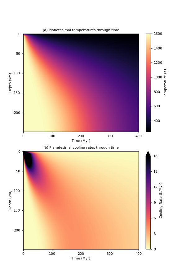
To get an overview of the cooling history of the body, it’s very useful to plot the temperatures and cooling rates as a heatmap through time. In order to plot the results, we need to define a figure height and width, then call load_plot_save.plot_temperature_history(), load_plot_save.plot_coolingrate_history() or load_plot_save.two_in_one(). These functions convert the cooling rate from K/timestep to K/Myr to make the results more human-readable.

fig_w = 6
fig_h = 9

pytesimal.load_plot_save.two_in_one(
    fig_w,
    fig_h,
    mantle_temperature_array,
    core_temperature_array,
    mantle_cooling_rates,
    core_cooling_rates,)

Results can be saved in the same way as for the constant and variable properties examples.